In this post we’ll iteratively improve on multiplying two random 1024 x 1024 float matrices, resulting in a 20x speedup on CPU. We’ll mostly focus on how different mathematical interpretations of matrix multiplication translate to vastly different outcomes on modern hardware, but we’ll also touch a bit on topics like multithreading and SIMD.
You can find the full code for benchmarking here.
Interpretation 1: inner product
There are many interpretions of matrix multiplication. The simplest is that given A @ B = C, each element C[i,j] is the inner product between row A[i,:] and column B[:,j].
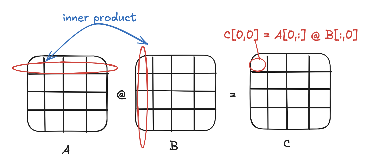
The implementation is also the simplest: the first loop iterates through the rows of A, the second loop iterates through the columns of B, the third loop iterates through the columns of A (and rows of B) and calculates the inner product. Here’s an implementation in C++, with each matrix represented as a float array and stored in row-major order.
template <int rowsA, int colsA, int colsB>
float *matmul_naive(float *A, float *B) {
    float *C = new float[rowsA * colsB];
    float tmp;
    for (int rowA = 0; rowA < rowsA; ++rowA) {
        for (int colB = 0; colB < colsB; ++colB) {
            tmp = 0.0;
            for (int colA = 0; colA < colsA; ++colA) {
                tmp += A[rowA * colsA + colA] * B[colA * colsB + colB];
            }
            C[rowA * colsA + colB] = tmp;
        }
    }
    return C;
}
We can stick this in a wrapper function that times how long it takes on a 1024 x 1024 matrix.
#include <chrono>

// Runs and times f(A, B)
float *run_and_time(float*(*f)(float*, float*), float *A, float *B) {
    std::chrono::steady_clock::time_point begin =
        std::chrono::steady_clock::now();
    float *C = f(A, B);
    std::chrono::steady_clock::time_point end =
        std::chrono::steady_clock::now();
    std::cout << "time = " <<
        std::chrono::duration_cast<std::chrono::microseconds>
        (end - begin).count() <<
        "µs" << std::endl;
    return C;
}
Which we can run as
int dim = 1024;
float *A = randmat(dim, dim); // generates pseudo-random dim x dim matrix
float *B = randmat(dim, dim);
float *C0 = run_and_time(matmul_naive<1024, 1024, 1024>, A, B);
This initial run takes 3.71s.
Unfortunately, the simplest interpretation is also the worst in practice since it is oblivious to the CPU’s cache organization. The pain point is the inner-most loop, in which we iterate over all the rows of B. Since we are storing our matrices in row-major order, we discard an entire cache line on each iteration of the inner-most loop.
Interpretation 2: linear combination of rows
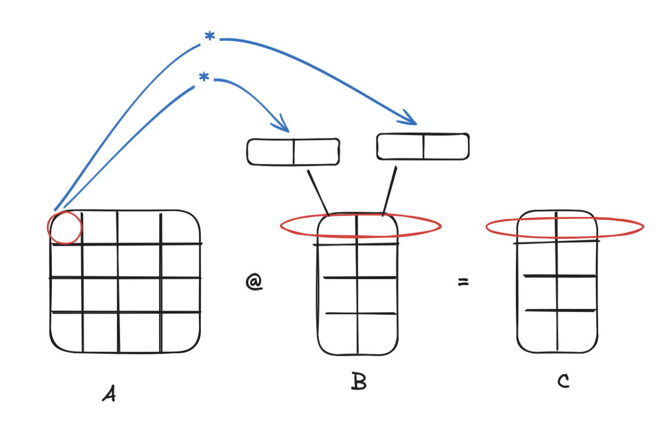
To fix this, recall from linear algebra an alternative interpretation of matrix multiplication: that each row of C, C[i,:], is a linear combination of all the rows of B, with the weights given by the columns of row A[i,:]. 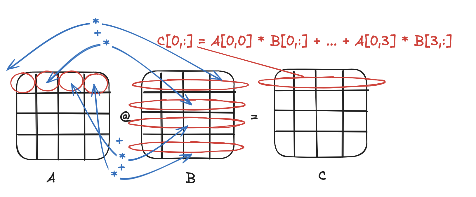
In other words,
C[i,:] = A[i,0] * B[0,:] + A[i,1] * B[1,:] + ... + A[i,n-1] * B[n-1,:]
Crucially, this means we don’t have to calculate each element of C to its entirety before moving on. We can calculate a partial result and come back to it on the next loop iteration. This allows us to use an entire cached row of B before moving on to the next. In code, this simply translates to a reordering of the two inner loops:
template <int rowsA, int colsA, int colsB>
float *matmul_loop_reordered(float *A, float *B) {
    float *C = new float[rowsA * colsB];
    for (int rowA = 0; rowA < rowsA; ++rowA) {
        for (int colA = 0; colA < colsA; ++colA) {
            for (int colB = 0; colB < colsB; ++colB) {
                C[rowA * colsA + colB] +=
                    A[rowA * colsA + colA] * B[colA * colsB + colB];
            }
        }
    }
    return C;
}
Which brings the time down to more than half our previous run of 1.62s.
However, we have yet another caching inefficiency. Observe that when we get to the next iteration i + 1 of the outer-most loop, we need to load the very first row of B, i.e. B[0,:], again. But since B[0,:] was last used in the beginning of iteration i, it will likely no longer be in the cache.
Interpretation 3: sum of outer products
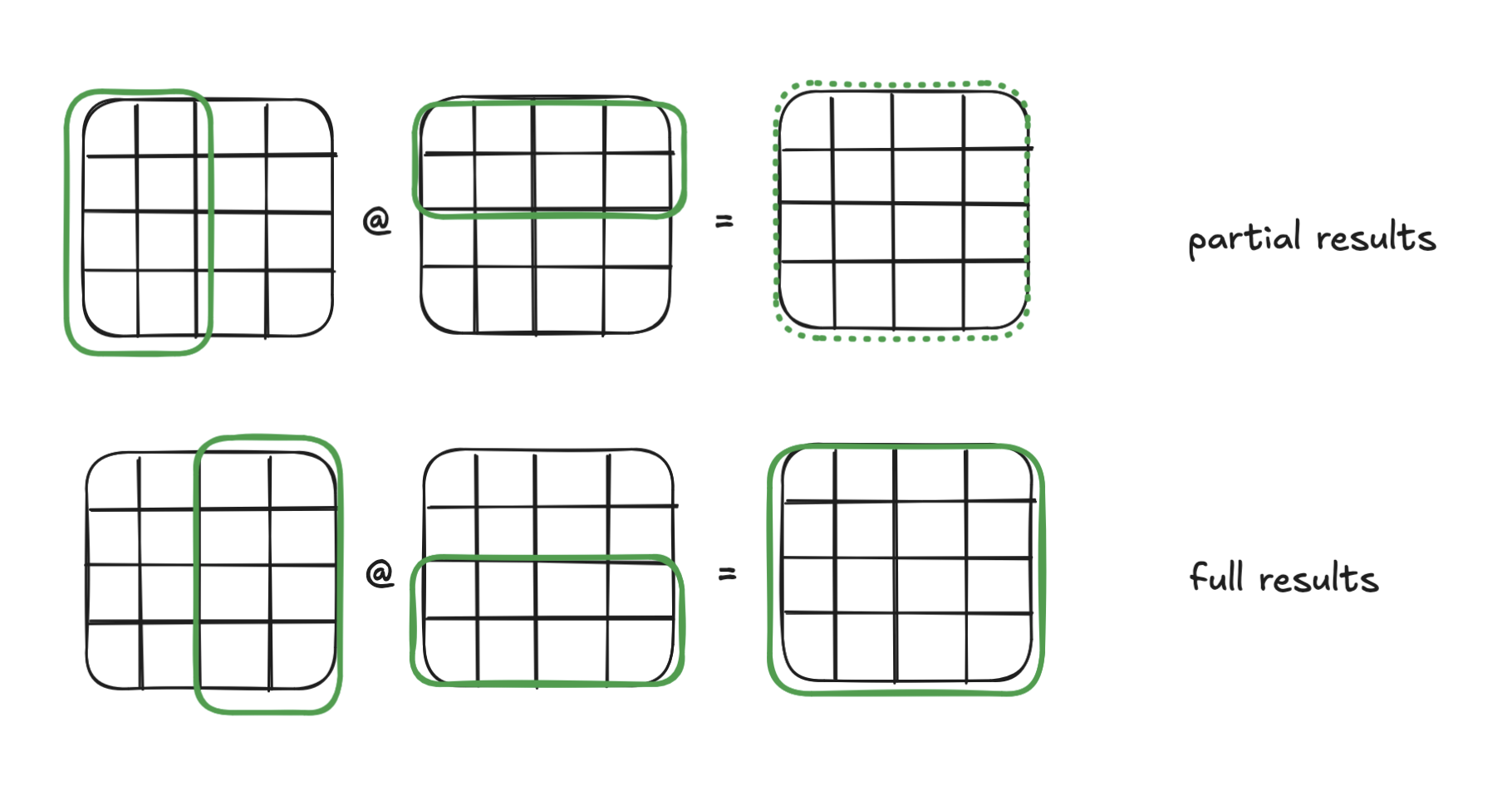
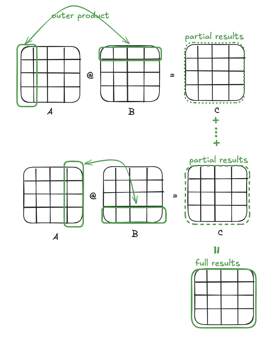
An interesting property of matrix multiplication is that you can take the outer product of any column of A and any row of B to get a partial result with the same dimensions as C. Add up all the partial results and you get the final result C. This is yet another interpretation of matrix multiplication: C can be viewed as a sum of all the outer products between the columns of A and rows of B.
To exploit this, we can divide our matrices into multiple tiles and run our previous algorithm on each of the tiles. Each tile run results in a intermittent result with the full dimensions of C. The final result is the sum of all the tile runs.
From a hardware standpoint, doing this ensures that we access the same elements close together in time, increasing the likelihood that they are still in the cache. For instance, when we reach iteration i + 1 of the outer loop, the first few rows of B will still be cached from the previous iteration i.
Choosing the correct tile size is non-trivial, but we can do some quick dirty math to estimate. We want to fit in the L1 cache:
- 1024 tiled row of A (1024 *
tile_size* 4B) tile_sizerows of B (tile_size* 1024 columns * 4B)- 1 full row of C (1024 * 4B)
The L1d cache size on my machine is 64KB, which means with a tile size of 4, we can keep 36896 bytes cached.
The implementation just adds an additional outer loop, and changes the inner loops to run on specific tiles rather than the whole of A and B.
template <int rowsA, int colsA, int colsB, int tile_size>
float *matmul_tiled(float *A, float *B) {
    float *C = new float[rowsA * colsB];
    // multiply A[:, tile * tile_size : (tile + 1) * tile_size]
    // and B[ tile * tile_size : (tile + 1) * tile_size ,:]
    for (int tile = 0; tile < colsA / tile_size; ++tile) {
        for (int rowA = 0; rowA < rowsA; ++rowA) {
            for (int colA = tile*tile_size; colA<(tile+1) * tile_size; ++colA) {
                for (int colB = 0; colB < colsB; ++colB) {
                    C[rowA * colsA + colB] +=
                        A[rowA * colsA + colA] * B[colA * colsB + colB];
                }
            }
        }
    }
    return C;
}
Unfortunately we don’t quite get a massive speedup we were hoping for; this runs for 1.60s. There’s probably other things going on that are polluting the cache, or maybe our matrices need to be much larger for tiling to have an significant impact.
Multithreading
So far we have only utilized one core, but we can vastly speed up our computation by dividing our work into multiple pieces. We just need to make sure the different pieces of work don’t have any dependencies between each other.
Luckily, matrix multiplication is quite suited for divide-and-conquer approaches, since any submatrix of C C[start_row:end_row,start_col:end_col] depends only on the corresponding rows of A and columns of B, i.e. A[start_row:end_row,:] and B[:,start_col:end_col]. 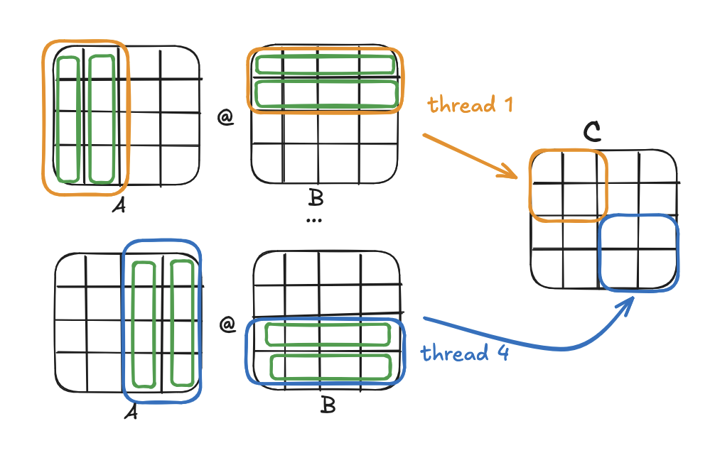
This means we can partition A and B into 2^n blocks and process each combination in a separate thread. With enough cores, in theory we should be able to achieve a 1/2^n speedup. Furthermore, as each thread writes to a separate section of C, we don’t need to worry about race conditions.
A function that computes some submatrix of C is known as a kernel. We can write one that takes the start and end rows and columns, computes the product submatrix, and writes to the appropriate section of C.
template <int rowsA, int colsA, int colsB, int tile_size>
void kernel(float *A, float *B, float *C,
        int start_row, int end_row, int start_col, int end_col) {
    for (int tile = 0; tile < colsA / tile_size; ++tile) {
        for (int rowA = start_row; rowA < end_row; ++rowA) {
            for (int colA=tile*tile_size; colA<(tile+1)*tile_size; ++colA) {
                for (int colB = start_col; colB < end_col; ++colB) {
                    C[rowA * colsA + colB] +=
                        A[rowA * colsA + colA] * B[colA * colsB + colB];
                }
            }
        }
    }
}
To make use of this, we just need to partition A and B, spin up multiple threads, and in each, call the kernel method on a specific combination of partitions.
template <int rowsA, int colsA, int colsB, int tile_size, int num_threads>
float *matmul_multithreaded(float *A, float *B) {
    float *C = new float[rowsA * colsB];
    int start, end;
    int block_size = rowsA / sqrt(num_threads);

    std::vector<std::thread> threads;
    int start_row, end_row, start_col, end_col;
    for (int row = 0; row < sqrt(num_threads); ++row) {
        start_row = row * block_size;
        end_row = row * block_size + block_size;
        for (int col = 0; col < sqrt(num_threads); ++col) {
            start_col = col * block_size;
            end_col = col * block_size + block_size;
            threads.push_back(
                std::thread(kernel<rowsA, colsA, colsB, tile_size>, A, B, C,
                    start_row, end_row, start_col, end_col)
            );
        }
    }
    for (auto &thread: threads) {
        thread.join();
    }
    return C;
}
With just 4 threads, our time improves to 0.46s.
Vectorization
Another way we can parallelize our code is to use SIMD instructions to speed up individual computations. For the sake of simplicity, we’ll use GCC’s SIMD extensions instead of dealing with intrinsics, but the latter is really what you want if you want reliability, as these extensions aren’t part of the C/C++ standard.
Anyhow, here’s how we can define a vector data type of 8 floats packed into a single register.
// 32 bytes for 8 floats
typedef float vec8 __attribute__ (( vector_size(32) ));

vec8 v = {1, 2, 3, 4, 5, 6, 7, 8};
v *= 2;
for (int i = 0; i < 8; ++i) {
    printf("%f ", v[i]);
}
> 2.000000 4.000000 6.000000 8.000000 10.000000 12.000000 14.000000 16.000000
Let’s forget about tiling and multithreading and go back to our loop-reordered example and see if we can improve it using SIMD vector extensions. Recall that we’re working with the row interpretation - that is, each row of C is a linear combination of rows of B, with the weights given by the columns of the corresponding row of A. We can collapse B and C into matrices of size rowsB * colsB / 8, where each element is a 8-float vector. Then, instead of doing colsB multiplications per row of B, we do colsB / 8 multiplications, where each is a vector instruction multiplying a scalar weight in A by a vector in B.
This is what the code looks like.
template <int rowsA, int colsA, int colsB>
vec8 *matmul_simd(float *A, float *B) {
    // setup: reshape B from colsA x colsB to colsA x colsB / 8
    vec8 *B_vec8 = new vec8[colsA * colsB / 8];
    vec8 tmp;
    for (int row = 0; row < colsA; ++row) {
        for (int col = 0; col < colsB / 8; ++col) {
            tmp = {
                B[row * colsB + col*8],
                B[row * colsB + col*8 + 1],
                B[row * colsB + col*8 + 2],
                B[row * colsB + col*8 + 3],
                B[row * colsB + col*8 + 4],
                B[row * colsB + col*8 + 5],
                B[row * colsB + col*8 + 6],
                B[row * colsB + col*8 + 7],
            };
            B_vec8[row * colsB / 8 + col] = tmp;
        }
    }

    // do the actual matmul
    vec8 *C_vec8 = new vec8[rowsA * colsB / 8];
    for (int rowA = 0; rowA < rowsA; ++rowA) {
        for (int colA = 0; colA < colsA; ++colA) {
            for (int colB = 0; colB < colsB / 8; ++colB) {
                C_vec8[rowA * colsB / 8 + colB] +=
                    A[rowA * colsA + colA] * B_vec8[colA * colsB / 8 + colB];
            }
        }
    }
    return C_vec8;
}
Running this on the same 1024 x 1024 matrix takes just 0.24s, without any multithreading or tiling! Redefining our vector type as
typedef float vec16 __attribute__ (( vector_size(64) ))
(16-float vectors) goes even faster, finishing in just 0.18s. You can pack as many floats as the maximum register width your processor supports.
This is just the tip of the iceberg; there are myriad other ways you can redesign your algorithm to exploit SIMD parallelism. Ultimately the name of the game is the fused multiply-add instruction, which multiplies two vectors and adds the result to a third vector - the core or matrix multiplication - all in a single step.
To sum it all up, here’s the final results on multiplying two 1024 x 1024 random matrices:
| algorithm | time |
| naive (inner products) | 3.71s |
| loop-reordered (linear combination of rows) | 1.62s |
| loop-reordered + tile size 4 | 1.60s |
| loop-reordered + tile size 4 w/ 4 threads | 0.46s |
| loop-reordered w/ SIMD (vec8) | 0.24s |
| loop-reordered w/ SIMD (vec16) | 0.18s |